Attention is 1/3 of All You Need

Since LLMs seem to be all the hype these days, I decided it was time to learn how the underlying components worked. Thanks to 3Blue1Brown, Neel Nanda, and Andrej Karpathy’s breakdown, I gained some high level intuition on transformers and wanted to solidify my understanding by re-explaining it here. There is nothing I have seen better than 3Blue1Browns visual explanation here. The other two links give a walkthrough of the code from scratch: Nanda and Karpathy.
How do we represent language in a deep learning model? Since neural networks are basically a glorified compilation of statistics and linear algebra, we must translate our language using beautiful things like vectors, matrices, and tensors. Really, all that goes on in any LLM/deep learning architecture is pretty much a bunch of these elements interacting with one another, as you will soon see in this article.
Tokenization & Embeddings
First, words in a sentence are broken down into smaller subparts called “tokens”, which essentially help capture more nuanced relationships between letters (for instance, “th” is more likely to be found than “tz” in the english alphabet, so “th” could be a likely candidate for a token). In reality, tokens are weird and messy, but all we need to know is that there are already learned dictionaries containing possible tokens in the English language, so we won’t need to worry too much about the details of how to break down words. The next step is to transform these tokens into numerical representations that a model can understand. This is where vector embeddings come in. Each token is mapped to a high-dimensional vector in a continuous space (using techniques like Word2Vec). These embeddings can ultimately capture semantic relationships between words, so vectors for “girl” and “boy” would be closer to each other than something like “girl” and “car”. When dealing with sentences, the order clearly matters, so positional embeddings are later added to the original embedding to encode for the unique position of each token in the sequence. Positional embeddings use cosine and sin functions to provide each token position with a unique vector.
A Single Layer of Attention
So we have represented words as tokens as vectors. Now, how does a transformer actually learn and predict the next words in a sequence? A transformer block consists of an attention layer and an MLP layer. Let’s start by seeing how the attention layer works.
For each token in a sequence, an attention score is calculated, which essentially helps encode the meaning of each word based on the context in the presence of other words. These attention scores are calculated over all possible pairs of tokens. Let’s use the following sentence as an example: “Greasy fried noodles will be my lunch”. The word “fried” in the context of “noodles” will be different from the word “fried” in a sentence like “Sherry fried in the sun”. However, the model initially has no idea that the semantic of “fried” should be in the context relevant to “noodles”, so by default, we should equally test out all possible pairs — “fried” and “will”, “fried” and “be”, “fried” and “lunch”, etc, to calculate an attention score for each token.
Exactly how are these attention scores calculated? There are three essential elements in computing the attention for each token: a query vector Q, key vector K, and a value vector V. The query and key vectors Q and K are produced after multiplying each token’s embedding with some learned weights matrices W_Q and W_K . You can think of the query vector as something that encodes some possible “question” about each token (which may or may not be relevant to the context as a whole). Then, each key vector encodes the “answer” to each token that reveals the extent to which it is relevant to the question in context. Taking the dot product (measure of similary) of the query and key vector, we get our attention scores for each token pair. Large positive attention weights indicate highly relevant word pairs, whereas negative values mean they are unrelated.
Masking
However, during training, if the model already knows what words come next in the sequence, it can easily just “cheat” and use the later words to go back and influence the weights of earlier words. So to prevent this, the model should be restricted such that it can only look forwards, and consider only how previous words can influence later words. Looking at the above matrix of attention scores between query-key vectors for each token pair, we should then only consider values in the upper triangular matrix, and ignore the entries in the lower left half. This basically just means that we don’t want a token in the 4th position to influence a token in the 1st, 2nd or 3rd position. This is a process called “masking”. In practice, we set the scores in the lower diagonal of the grid to negative infinity, and then take the softmax of each column. The softmax function just converts some number into a probability value ranging between 0 and 1, so that the columns can sum to 1.
These attention scores tell us the pattern of which previous words influence later words. But how exactly do we integrate this knowledge in order to update the original token embeddings (i.e., how can we carry over the meaning of “fried” into the word it describes “noodle”)? This is where the value vector V comes in, which essentially acts as a weight for the attention score, (i.e., the extent to which previous words should actually influence the current word). V is produced by multiplying each token’s original embedding by some learned value matrix W_V . Next, we multiply the V with the attention score for each token, and then sum up the values in each column that essentially produces some new vector that we can add onto the original embedding. Basically, this new vector encodes all the relevant information from previous words that can influence the context of the current word. The new updated embedding for each token is equal to the original embedding plus this new vector.
Multilayered Attention
Everything above describes only a single layer of attention (one attention head). But typically, there are many layers of attention within the attention block. In theory, each query, key, and value vector encodes one possible contextual cue (i.e., “fried” being an adjective for the noun “noodles”), but in reality there are many other possibilities of how context and syntax can influence semantics. What happens in multi-headed attention is that many single attention heads run in parallel to capture a larger variety of patterns in language. In the case for GPT-3 there are 96 different attention layers, producing 96 new vectors to add onto the original token embedding .
MLP Layer
As the name of the original paper “Attention is All You Need” suggests, the most important part of a transformer is exactly this attention module. However, prefaced by the title of this article (shamelessly stolen from 3Blue1Brown’s explanation), attention is not all there is. The remaining 2/3 is largely the MLP layers that come after. But before the attention layer is fed into an MLP, the outputs go through a “LayerNorm” technique, which essentially is just a normalization approach using the mean and variance of features in each training input. After this step, the normalized outputs are passed on through to a fully connected MLP layer, which is what helps the model reason, compute, extract language patterns, etc. All information is retained in the “residual stream” which is where the model encodes previous information. It is the sum of all previous outputs, taken as an input to feed into the new layers. Repeat this iterative process for how ever many number of times, and in the end we are able to get a magical language model.


